View Tab and its Usage in Excel

What is View Tab ? Where is it in Excel ?

      This is the last Tab after Review Tab in Excel. Every tab has its own importance in Excel ribbon in which View tab helps to change the view of Excel sheet and make it easy to view the data. Also, this tab is useful for preparing the workbook for printing.
It looks like image below.

View Tab in Excel

It has Five Groups.
1. Workbook Views
2. Show/Hide
3. Zoom
4. Window
5. Macros

1. Workbook Views :

 Excel offers 4 types of workbook views: – Normal, Page break preview, Page layout & Custom View. 

Normal - View the document in Normal view.

Page Layout - View the document as it will appear on the printed page. Use this view to see where pages begin and end, and to view any headers or footers on the page.

Page Break Preview - View a preview of where pages will break when this document is printed.

Custom Views - Save a set of display and print settings as a custom view. Once you have saved the current view, you can apply it to the document by selecting it from the list of available custom views.


Full Screen - View the document in full screen mode.

2.Show / Hide:

We use this option to show and hide the Excel’s view. Ruler is used to show the rulers next to our documents. 

Ruler - View the rulers used to measure and line up objects in the document.

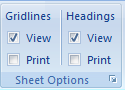
Grid lines - Show, or hide, the lines between rows and columns in the sheet. Showing makes numbers in columns or rows easier to read or edit. Hiding Grid lines is useful if you are making a graphic organizer in Excel. These lines will not print unless the Print box is checked.

Message Bar - Open the Message Bar to complete any required actions on the document.

Formula Bar - View the formula bar in which you can enter text and formulas into cells.

 Headings - Show row and column headings. Row headings are the row numbers on the side of the sheet that range from 1 to 1,048,576. Column headings are the letters that appear above the columns on a sheet that range from A to XFD. This is also found on the Page Layout tab of an Excel Workbook.

3.Zoom:

-We can adjust the view as per our convenience.

Zoom - Open the Zoom dialog box to specify the zoom level of the document. In most cases, you can also use the zoom controls in the status bar at the bottom right portion of the window to quickly zoom the document.

100% - Zoom the document to 100% of the normal size.

Zoom to Selection - Zoom the worksheet so that the currently selected range of cells fills the entire window. This can help you to focus on a specific area of the worksheet.

4.Window :

We use this option to access the window options. 

New Window - Open a new window containing a view of the current document.

Arrange All - Tile all open program windows side-by-side on the screen.   

Freeze Panes - Keep a portion of the sheet visible while the rest of the sheet scrolls.   

Reset Window Position - Reset the window position of the documents being compared side-by-side so that they share the screen equally. To enable this feature, turn on View Side by Side.

Split - Split the window into multiple resizable panes containing views of your worksheet. You can use this feature to view multiple distant parts of your worksheet at once.

Save Workspace - Save the current layout of all windows as a workspace so that it can be restored later.

 Hide - Hide the current window so that it cannot be seen. To bring the window back, click the Unhide button.

Switch Windows - Switch to a different currently open window.

  

Unhide - Unhide and windows hidden by the Hide Windows feature.

View Side by Side - View two worksheets side-by-side so that you can compare their contents.

Synchronous Scrolling - Synchronize the scrolling of two documents so that they scroll together. To enable this feature, turn on View Side by Side.

5. Macros

With this option, we can record the macro and then we can view the macro.

 View the list of macros, from which you can run, create, or delete a macro. The keyboard shortcut for viewing macros is 

Alt + F8 .

Review Tab and its Usage in Excel

What is Review Tab ? Where is it in Excel ?

     In Excel Riview Tab is after Data. Review tab contains the editing feature, comments, track changes and workbook protection options. These features make it easy to share the data with the proper information whilst ensuring security of data.

It looks like Image below.

Review Tab 

In MS Excel 2007 It is divided in three parts.

1. Proofing

2. Comments

3. Changes

Parts of Review Tab

1. Proofing:

We use proofing to correct the typo mistakes through spelling option. Research and dictionary work alike, to translate the sentence in any other language.. And Thesaurus suggests other ways to say anything.

Proofing in Excel

Spelling - Check the spelling of text. The keyboard shortcut to check spelling is F7.

Research - Open the Research Task Pane to search through reference materials such as dictionaries, encyclopedias, and translation services. The keyboard shortcut for Research is Alt + Click.

Thesaurus - Suggests other words with a similar meaning to the word you have selected.

Translate - Translate the selected text into a different language.

2. Comments:

When we want to give the message about the cell, we use comment option. We can insert and delete the comment, show and hide the comment, and then we have an option to show all the comments.

Comment Tab in Excel

Edit Comment - Edit the selected comment. The keyboard shortcut to edit a selected comment is Shift + F2 . Note: This button will not be displayed unless a cell containing a comment has been selected.

New Comment - Add a comment about the selected cell. The keyboard shortcut to add a comment is Shift + F2 . Note: This button is the default view in the Comments section rather than the Edit Comment button displayed at the top of this explanation.

Delete (comment) - Delete the selected comment.

Previous (comment) - Select the previous comment in the worksheet.

Next (comment) - Navigate to the next comment in the document.

Show/Hide Comment - Show or hide the comment attached to the selected sheet.

Show All Comments - Display all comments in the sheet.

Show Ink - Show or hide any ink annotations on the sheet.

3. Changes:

We use Changes option to protect the sheet and workbook, and we can allow user to edit the specific range; also, we can share the workbook as well. 

Changes Tab in Excel

Protect Sheet - Prevent unwanted changes to the data in a sheet by specifying what information can be changed. For example, you can prevent people from editing locked cells or changing the formatting of the document. You can specify a password that can be entered to unprotect the sheet and allow these changes.

Protect Workbook - Prevent unwanted changes to the structure of the workbook, such as moving, deleting, or adding sheets. You can specify a password that can be entered to unprotect the workbook and allow these changes.

Share Workbook - Allow multiple people to work in a workbook at the same time. The workbook should be saved to a network location where multiple people can open it. Workbooks containing tables cannot be shared.

Protect and Share Workbook - Share the workbook and protect it with a password at the same time. The password will prevent others from turning off change tracking.

Allow Users to Edit Ranges - Allows specific people to edit ranges of cells in a protected workbook or sheet. Before using this feature, first set security on the sheet by using the Protect Sheet command. To use this feature, your computer must be joined to a Microsoft Windows domain.

Track Changes - Track all changes made to the document, including insertions, deletions, and formatting changes.

Data Tab and its usage in Excel

What is Data Tab ? Where is it in Excel ?

        Data tab is another most important part of excel. It is between Formulas Tab and Review Tab. We use Data tab for the large amount of data.It is useful to import the data by connecting with the server, and we can import data automatically from web, MS Access etc. And sort & filter are very helpful options we have in Excel; it makes easy to read vast data.
It looks like  imagae below.

Data Tab

Data Tab is Divided in to Five Group.
1. Get External Data
2. Connections
3. Sort & Filter
4. Data Tools
5. Outline

1. Get External Data:

 In Excel, we can import data from MS Access, Web, Text and other sources. Also, we can import the data from other applications.

From Access - Import data from a Microsoft Access database.

From Web - Import data from a web page.

From Text - Import data from a text file.

From Other Sources - Import data from other data sources.

Existing Connections - Connect to an external data source by selecting from a list of commonly used sources.

2. Connections:

      It is used to display the entire data connections for the workbook. Data connections are links to the data outside the workbook which can be updated if the source data changes. And updated data can be obtained by refreshing all sources in workbook.

Refresh All - Update all the information in the workbook that is coming from a data source. The keyboard shortcut to Refresh All is Ctrl + Alt + F5 .

Connections - Display all data connections for the workbook. Data connections are links to data outside of this workbook which can be upgraded if the source data changes.

Properties - Data Range Properties - Specify how cells connected to a data source will update, what contents from the source will be displayed, and how changes in the number of rows or columns in the data source will be handled in the workbook.

Edit Links - This is used to break a link to an external reference. This command will be unavailable if the workbook does not contain linked information.

3. Sort & Filter:

To set the data in ascending or descending order on the basis of value or as per the first letter of a word, we use Sort option. Also, we can put the basic and advanced filter from here only.

Sort A to Z - Sort the selection so that the lowest values are at the top of the column.

Sort Z to A - Sort the selection so that the highest values are at the top of the column.

Sort - Launch the Sort to sort data based on several criteria at once.

Filter - Enable filtering of the selected cells. Once filtering is turned on, click on the arrow in the column header to choose a filter for the column. The keyboard shortcut to filter is Ctrl + Shift + L.

Clear - Clear the filter and sort data for the current range of data.

Reapply - Reapply the filter and sort in the current range. New or modified data in the column won't be filtered or sorted until you click Reapply. The keyboard shortcut to reapply is Ctrl + Alt + L.

Advanced - Specify complex criteria to limit which records are included in the result set of a query.

4. Data Tools:

This option is very important to make the report interactive; it helps us to make the data authentic, and using this tab, we can restrict or validate the entries if the data is being updated by multiple users. Text to Columns helps us to split the single column into multiple columns as per data. Flash fills the values in the range. We can delete duplicate rows from the data by using Remove Duplicates option. We use Data Validation to provide the list that can be entered in cell, or we can restrict the entries, or we can validate the entries in the cell. We use Consolidate option to summarize data from separate ranges, and consolidate the result in a single output range. We use What-if-Analysis to analyse the data.

Text to Columns - Separate the contents of one Excel into separate columns. For example, you can separate a column of full names into separate first and last name columns. In Word you would use this feature to convert the selected text into columns at each comma, period, or other character you specify.

Remove Duplicates - Delete duplicate rows from a sheet. You can specify which columns should be checked for duplicate information.

Data Validation - Prevent invalid data from being entered into a cell. For example, you could reject sates or numbers greater than 1000. You can also force input to be chosen from a dropdown list of values you specify.

Consolidate - Combine values from multiple ranges into one new range.

What-If Analysis - Try out various values for the formulas in the sheet. Scenario Manager allows you to create and save different groups of values, or scenarios, and switch between them. Goal Seek will find the right input when you know the result you want. Data Tables allow you to see the results of many different possible inputs at the same time.

5. Outline:

We use this option to make the data more analytical and understandable. We can make group of rows or columns or automatically create an outline. We can ungroup the data; quickly calculate rows of related data by inserting subtotals and totals. We use Show and Hide options when we want to insert the Subtotal in data.

Group - Tie a range of cells together so that they can be collapsed or expanded. The keyboard shortcut to Group is Shift + Alt + Right.

Ungroup - Ungroup a range of cells that were previously grouped. The keyboard shortcut to Ungroup is Shift + Alt + Left.

Subtotal - Total several rows of related data together by automatically inserting subtotals and totals for the selected cells.

Show Detail - Expand a collapsed group of cells.

Hide Detail - Collapse a group of cells.

Diagonal Arrow - Click on the arrow in the bottom right corner of Outline to see the Settings dialog box.
If you liked our blogs, share it with your friends on Facebook. And  Twitter. We would love to hear from you, do let us know how we can improve, complement or innovate our work and make it better for you. Please Comment in on the post.

Formula Tab and its Ussage in Excell

What is Formula Tab ? Whare is it in Excel ?

    Formula Tab is the most important part of Excel. It is between the Page Layout Tab and Data. We use Formula tab to insert functions, define the name, create the name range, review the formula, etc. In ribbon, Formulas tab has very important and most useful functions to make dynamic reports.

It looks like image below.

It is divided in Four part.

1. Function Library

2. Defined Names

3. Formula Auditing

4. Calculation

1.  Function Library: 

        In Excel, we have 461 functions and they are available in the formulas tab under the function library group. And there is no need to learn every formula for we can find formulas category wise such as:- Financial, Logical, Text, Date & Time, Lookup & Reference, Math & Trig, many more. We will must Discuss this in detail in another article.

Insert Function - Edit the formula in the current cell by choosing functions and editing the arguments. The keyboard shortcut to insert a function is Shift + F3 .

AutoSum - Display the sum of the selected cells directly after the selected cells. The keyboard shortcut for autosum is Alt + = .

Recently Used - Browse and select from a list of recently used functions.

Financial - Browse and select from a list of financial functions.

Logical - Browse and select from a list of logical functions.

Text - Browse and select from a list of text functions.

Date and Time - Browse and select from a list of date and time functions.

Lookup and Reference - Browse and select from a list of lookup and reference functions.

Math and Trig - Browse and select from a list of math and trigonometry functions.


More Functions - Browse and select from lists of statistical, engineering, cube, and information functions.

2.  Defined Names: 

       We use this option to define the name of a cell, range and the list of the already defined name can be viewed in Name manager and we can edit it if we want to change the range or cell reference of any defined name. Also, we can use the defined name in Formulas.

Name Manager - Create, edit, delete, and find all the names used in the workbook. The keyboard shortcut to access the name manager is Ctrl + F3.

Defined Name - Name cells so that you can refer to them in formulas by that name. For example, you might name the cells A20 to A40 "Expenses." Names can be used in formulas to make them easier to understand.

Use in Formula - Choose a name used in the workbook and insert it into the current formula.


Create from Selection - Automatically generate names from the selected cells. Many people choose to use the text in the top row or the leftmost column of a selection. The keyboard shortcut to create from selection is Ctrl + Shift + F3 .

3.  Formula Auditing: 

        This option helps us to identify the relation of formulas. By using Trace precedent, we get to know on which cell formula cell is based. Trace dependents are used to know if active cell is being used in any formula. When we use trace precedent and trace dependents the arrows get inserted automatically and, to remove the arrows, we use Remove Arrows. Show formula is a self-explained word; it is used to show the formula in the sheet. Error checking is used to check the error in the sheet. Evaluate formula option is used to evaluate the formula step by step.

Trace Precedents - This will show arrows that indicate what cells affect the value of the currently selected cell.

 Trace Dependents - This will show arrows that indicate what cells are affected by the value of the currently selected cell.

Remove Arrows - This will remove the arrows drawn by Trace Precedents or Trace Dependents.

Show Formulas - Display the formula in each cell instead of the resulting value. The keyboard shortcut to show formulas is 
Ctrl + ' \.

Error Checking - Check for common errors that occur in formulas.

Evaluate Formula - Launch the Evaluate Formula dialog box to debug a formula by evaluating each part of the formula individually.


Watch Window - Monitors the values of certain cells as changes are made to the sheet. The values are displayed in a separate window that remains visible, regardless of what area of the workbook is shown.

4.  Calculation: 

      If we want to switch the calculation from automatically to manually calculation and manually to automatically calculation, then we can do it by using the Calculation option. We use Calculate Now and Calculate Sheet option if automatic calculation is turned off.

Calculation Options - Specify when formulas are calculated. By default, any time you change a value that affects other values, the new values are calculated immediately.

Calculate Now - Calculate the entire workbook now. This is only necessary if automatic calculation has been turned off. The keyboard shortcut to calculate now is F9 .


Calculate Sheet - Calculate the current sheet now. This is only necessary if automatic calculation has been turned off. The keyboard shortcut to calculate sheet is Shift + F9 .

If you liked our blogs, share it with your friends on Facebook. And  Twitter. We would love to hear from you, do let us know how we can improve, complement or innovate our work and make it better for you. Please Comment in on the post.

Page Layout Tab and its ussege in Excel

What is Page Layout Tab ? Whare is it in Excel ?

      Page Layout Tab is Just Near the Insert Tab. In Page Layout option, we have various commands which we use to prepare the workbook for printing and exporting to PDF format. Through this command, we can adjust the page in the way we want to see after printing.

It  Looks Like image below

In Page Layout Tab We have five group

1. Theme

2. Page Setup

3. Scale to Fit

4. Sheet Options

5. Arrange

1. Theme

      This option is used to change the theme color of workbook by just click of a button. Each theme has 12 colors, two fonts (heading and body), SmartArt and the effects for shape. Also, we have color option whereby we can create new color’s theme, by using the Font option, we can create new font theme as well. So, if we want to create our own theme we can create it by using Themes option in Excel.  Themes - Change the overall design of the entire document, including colors, fonts, and effects.

Colors - Change the colors for the current theme.

Fonts - Change the fonts for the current theme.


Effects - Change the effects for the current theme.

2. Page Setup

    We use this option to set up the page for printing. So, we have Margins, Orientation, Size, Print Area, Breaks, Background and Print titles, in this group, which we use to prepare the page for printout.

Margins - Select the margin sizes for the entire document or the current selection.

Orientation - Switch the pages between portrait and landscape layouts.

Size - Choose a paper size for the current section. To apply a specific paper size to all sections of the document, click on More Paper Sizes .

Print Area - Mark a specific area of the sheet for printing.

Breaks - Specify where a new page will begin in the printed copy. Page breaks are inserted above and to the left of the selection.

Background - Choose an image to display as the background of a sheet.

Print Titles - Specify rows and columns to repeat on each printed page.

Diagonal Arrow - Click on the arrow in the bottom right corner of Page Setup to see the Page Setup dialog box (Page tab selected, three other tabs are available.)

3. Scale To Fit.

 

 This option helps to fit the page for printing by shrinking or enlarging its size to better fit the pages. We can use Scale to fit to adjust the width and height by describing the scale %age.

Width - Shrink the width of printed output to fit a maximum number of pages.

Height - Shrink the height of printed output to fit a maximum number of pages.

Scale - Stretch or shrink the printed output to a percentage of its actual size. The maximum width and height must be set to "Automatic" to use this feature.

Diagonal Arrow - Click on the arrow in the bottom right corner of Scale to Fit to see the Page Setup dialog box (Page tab selected, three other tabs are available)

4. Sheet Option

It is also a printing option that can show or hide the gridlines, while printing and heading options are used to give headings to the rows and columns.

Gridlines - Show, or hide, the lines between rows and columns in the sheet. Showing makes numbers in columns or rows easier to read or edit. Hiding gridlines is useful if you are making a graphic organizer in Excel. These lines will not print unless the Print box is checked.

Headings - Show row and column headings. Row headings are the row numbers on the side of the sheet that range from 1 to 1,048,576. Column headings are the letters that appear above the columns on a sheet that range from A to XFD. This is also found on the View tab of an Excel Workbook.

5. Arrange

          We use this option to arrange the objects back and forward and align it. Also, we have Selection pane option by which we can see total images in the workbook and select them from there.

Bring to Front - Bring the selected object in front of all other objects so that no part of it is hidden behind another object.

Send to Back - Click here to send the selected object back one level or to the back of all objects.

Selection Pane - Show the Selection Pane to help select individual objects and to change their order and visibility.

Align - Align the edges of multiple selected objects. You can also center the objects or distribute them evenly across the page.

Group - Group objects together so that they can be treated like a single object.


Rotate - Rotate or flip the selected object.

If you liked our blogs, share it with your friends on Facebook. And  Twitter. We would love to hear from you, do let us know how we can improve, complement or innovate our work and make it better for you. Please Comment in on the post.

Insert Teb and Its ussage in Excel

What is Insert Teb ? Where is It In Excel ?

Insert Tab is just near the Home Teb, it is useful to insert the picture, charts, filter, hyperlink etc. We use this option to insert the objects in Excel. To open the insert tab, press shortcut keys Alt+N.

It looks like below

Insert teb https://parthexcelmaster.blogspot.com

Insert Teb is divided in 5 Group:

1. Table

2. llustrstion 

3. Chart

4. Link

5. Text

1. Table

         Pivot Table - Summarize data using a Pivot Table. Pivot Table makes it easy to arrange and summarize complicated data and drill down on details.

       Table - Create a table to manage and analyze related data. Tables make it easy to sort, filter, and format data within a sheet. You can also use the keyboard shortcut Ctrl + T to create a table.

2. Illustration

Picture - Insert a picture from a file.

Clip Art - Insert Clip Art into the document, including movies, sounds, or stock photography to illustrate a specific concept.

Shapes - Insert ready-made shapes, such as rectangles and circles, arrows, lines, flow chart symbols, and callouts.

SmartArt - Insert a Smart Art graphic to visually communicate information. Smart Art graphics range from graphical lists and process diagrams to more complex graphics, such as Venn diagrams and organization charts. Caution ! Using the SmartArt version of a Venn diagram does not make use of everything you may want to do with a Venn. For example, you can not type in the overlap area where you normally place shared characteristics of the things you are comparing. To make a true Venn you should use the circle tool in Shapes .

3. Charts

Column - Insert a column chart. Column charts are used to compare values across categories. If chart data is selected, or the cursor is in or adjacent to the data, pressing F11 automatically creates a column chart.

Line - Insert a line chart. Line charts are used to display trends over time.

Pie - Insert a pie chart. Pie charts display the contribution of each value to a total. Use a pie chart when values can be added together or when you have only one data series and all values are positive.

Bar - Insert a bar chart. Bar charts are the best chart type for comparing multiple values.

Area - Insert an are chart. Area charts emphasize differences between several sets of data over a period of time.

Scatter - Insert a Scatter chart, also known as an X Y chart. This type of chart compares pairs of values. Use a Scatter chart when the values being charted are not in X-axis order or when they represent separate measurements.

Other Charts - Insert a stock, surface, doughnut, bubble, or radar chart.

Diagonal Arrow - Click on the arrow in the bottom right corner of Charts to see the Insert Chart dialog box to see all of the available charts.

4. Link

Hyperlink - Create a link to a Web page, a picture, an e-mail address or a program. You can also use the keyboard shortcut Ctrl + K to create a hyperlink.

5. Text

Text Box - Insert a text box that can be positioned anywhere on the page. In Office 2007 you can also create a text box by using the Paste as Picture feature when on the Home tab.

Header & Footer - Edit the Header or Footer of the document. The information in the Header or Footer will appear at the top or bottom of each printed page.

 WordArt - Insert decorative text in your document. Caution : if you are a long-time user of Word Art you may be a bit disappointed in the 2007 version - the choices are a bit tame.

Signature Line - INsert a signature line that specifies the individual who must sign. Inserting a digital signature requires that you obtain a digital ID, such as one from a certified Microsoft partner.

Object - Insert an embedded object. Some objects supported are Adobe Acrobat documents, Photoshop Elements images, Microsoft Equation, and several others.

Symbol - Insert characters that are not on your keyboard, such as copyright symbols, trademark symbols, paragraph marks.

Unicode characters - This is way beyond Wingdings or Webdings. Even Times New Roman has a large number of symbols and foreign letter characters which can be inserted.

If you liked our blogs, share it with your friends on Facebook. And  Twitter. We would love to hear from you, do let us know how we can improve, complement or innovate our work and make it better for you. Please Comment in on the post.

Home Tab in Excel

What is Home Tab ? Where is it in Excel?

 This is First Tab.  Home tab contains the most frequently used options such as cut-copy-paste, font formatting, alignment, Number, Conditional formatting, etc. All the options are used to format the data.

It looks like below image in Excel.

Home Tab Parth Excel Master

In Excel it is divided in 7 Group
1.Clipboard
2. Font
3.Alignment
4. Number
5. Style
6. Cells
7. Editing
Above division is Explained in image below.

7 division of Home Tab

1. Clipboard

             This group contains frequently used commands: Cut, Copy, Paste and Format painter. Clipboard option allows us to collect text and graphic items and paste it.

        In Paste menu you can find Paste Speacial  It will be useful to paste Data without Formula or Other paste option with your choce.

2. Font

           We use this option to change the font style and font-size. We can make it bold, italic and underline. Also, this group contains border styles, fill color, font color. It is same in word and Excel both.

3. Alignment

            We use this option to change the alignment of cell’s text to the right, left and middle. Also, we can subject the text to top, bottom, and middle alignment. In this group, we have Wrap text option to adjust and make the text visible within a cell, and we can also merge 2 or more cells, using merge option.

It also somewhat similar like word, but there are some functions like Wrap Text and Merge and Centre, Decrease Indent and Increase Indent are very useful to work with numbers. 

4. Number

     We use this option to change the number formatting into General, Percentage, Currency, Date, Time, Fraction etc. We can increase and decrease the decimal and convert the number into accounting number.

  

5. Style

          In this option, we have Conditional Formatting, Format as Table and Cell Styles. Conditional formatting is used to highlight the cell or range on the basis of conditions. Format as table is having readymade table format and Cell styles feature different types of built-in styles that are a combination of Font style, Font color and Fill color. You can decorate your sheet.

Conditional Formatting

Format as Table

Cell Styles

6. Cells

     We use this option to insert or delete cells, rows, columns and sheets. Also, we have format option to adjust the height, width of cells or range. Using this option, we can hide or unhide the range, protect the workbook, rename the sheet name, fill the tab color, move or copy to sheets, lock the cells.

                             

7. Editing

       This option has Auto Sum feature to return the total of numbers and move the text to right, left, up and down, Clear the format, content, comments and hyperlink; sort the data and find and select option.

If you liked our blogs, share it with your friends on Facebook. And  Twitter. We would love to hear from you, do let us know how we can improve, complement or innovate our work and make it better for you. Please Comment in on the post.

Thanks to All